|
Power Regression Model Example
|
Side note: Power regressions will not allow an
independent variable value of zero.
This example does not utilize an independent variable
value of zero. |
|
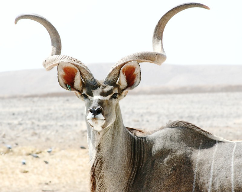
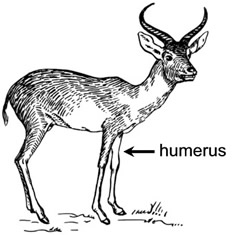
Antelopes are native to Africa and Asia. They range in size from
12" (30 cm. at the shoulder) pygmy antelopes to giant
elands,
which are over 6 feet tall (180 cm) at the shoulder.
Most antelopes are between 3 to 4 feet tall (90-120 cm) at the shoulder. The horns of antelopes, unlike
the antlers of deer, are un-branched, are made of a
shell with a bony core, and are not shed.
The majority of antelopes reside in Africa.
The kudus antelope, shown here, relies on thickets for protection using his brown and striped coat as camouflage. |
|
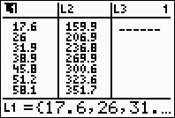
Data: The data below represents the length and mid-shaft diameters
of the humerus bones of African Antelopes.
| Diameter (mm) |
Length (mm) |
| 17.6 |
159.9 |
| 26.0 |
206.9 |
| 31.9 |
236.8 |
| 38.9 |
269.9 |
| 45.8 |
300.6 |
| 51.2 |
323.6 |
| 58.1 |
351.7 |
| 64.7 |
377.6 |
| 66.7 |
384.1 |
| 80.8 |
437.2 |
| 82.9 |
444.7 |
|
| Task: Express
answers to the nearest tenth. |
| |
a.) |
Prepare a scatter plot of the data. |
| |
b.) |
Determine a power
regression model equation to represent this data. |
| |
c.) |
Graph the new
equation. |
| |
d.) |
Decide whether the
new equation is a "good fit" to represent this data. |
| |
e.) |
Extrapolate data:
What length will correspond to a diameter of 84 mm? |
| |
f.) |
Interpolate data: What length will correspond to a diameter of 47 mm? |
| |
g.) |
What mid-shaft diameter will correspond to a length of 305.7 mm? |
|
Step 1.
Enter the data into the lists.
For basic entry of data, see Basic
Commands. |
 |
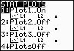
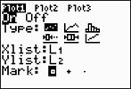
Step 2.
Create a scatter plot of the data.
Go to STATPLOT (2nd Y=)
and choose the first plot. Turn the plot
ON, set the icon to Scatter
Plot (the first one), set Xlist
to L1 and Ylist to
L2 (assuming that is where
you stored the data), and select a Mark of your choice.
  |
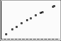
(answer to part a)
|
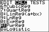
Step 3.
Choose the Power Regression Model.
Press STAT, arrow right to
CALC, and arrow down to
A: PwrReg. Hit
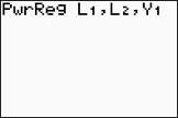
ENTER. When
PwrReg appears on the home
screen, type the parameters L1,
L2, Y1. The Y1
will put the equation into Y=
for you. (Y1 comes from VARS → YVARS, #Function, Y1)
|
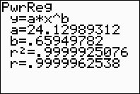
The power regression equation is

(answer to part b)
|
Step 4.
Graph the Power Regression Equation from
Y1.
ZOOM #9 ZoomStat to see
the graph. |
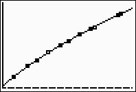
(answer to part c)
|
Step 5.
Is this model a "good fit"?
The correlation coefficient, r, is .9999937121
which indicates a very strong correlation since it is
close to 1.
The coefficient of determination, r
2, is .99999250766 which means
that 99% of the total variation in y can be
explained by the relationship between x and y.
Yes, it is a very "good fit".
(answer to part d) |
|
Step 6.
Extrapolate:
(beyond the data set)
Go to TBLSET (above WINDOW)
and set the TblStart to 84. Notice how setting the increment (the deltaTbl = 0.1) displays certain values to two decimal places. The calculator is trying to tell you that this value has been "rounded" to the nearest hundredth and should not be now rounded to the nearest tenth.
Always check the "full" Y1 value, as seen at the bottom of the screen, before rounding.
(See an alternate method in Step 7.)
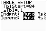 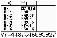
(answer to part e - the length will be 448.3 mm) |
Step 7.
Interpolate:
(within the data set)
From the graph
screen, hit TRACE, arrow up
to obtain the power equation, type 47, hit ENTER, and
the answer will appear at the bottom of the screen. 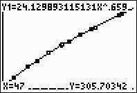
(answer to part f - length will be 305.7 mm) |
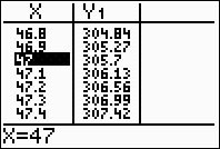
Step 8. What mid-shaft diameter will correspond to a length of 305.7 mm?
In reference to the equation, go to TABLE (above GRAPH)
and arrow down until you find a Y1 value equal to (or close to) the desired value. The answer will appear in the X column. (answer to part g - 47 mm. |
|
|