To insert a page for lists and spreadsheets, choose option #3 Lists and Spreadsheets from the HOME screen or press CTRL I (to choose the insertion of a spreadsheet page). This spreadsheet behaves much like Microsoft Excel.
Remember, you MUST name your lists!
Remember, to do a formula, you must start with an equal sign (=).
EXAMPLE:
Consider the data set: {15, 22, 32, 31, 52, 41, 11}
We will name this data set Ex1.
Entering Data:
Simply type your data and press ENTER after each entry, or arrow down. Use your arrows to move between cells and columns.
You MUST Name your list: Arrow to the top of the column and enter the name of your list. Keep the name descriptive, but short. We are naming our list Ex1, for this first example.
You can edit a cell entry by typing over it.
You can delete a cell entry by highlighting the cell and pressing CTRL-MENU, #1 Cut. |
|
| Creating a new list: Data can be entered in a second list based upon the information in a previous list. We will now double all of our data values in Ex1 and store them in column B, which we will name Twice. Arrow over to the shaded cell below the listing of column B. Type the formula = 2 * Ex1 into this cell. The formula will also appear at the bottom of the screen. Press ENTER and the new list is created. |
|
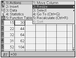
Resizing the Columns: Often times it is necessary to make a column wider so that you can more clearly see its contents.
1. Move to a cell in the column you wish to adjust.
2. Hit MENU, #1 Actions, #2 Resize, #1 Resize Column Width
3. Use your arrow to drag the edge of the column to the right to enlarge the column.
4. Resize row height by highlighting the row and then follow the menu options again.
The columns are now wider and the formula is more easily viewed.
|
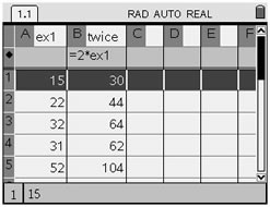
|
Delete or Clear a Column: To delete or clear a column, arrow to the top of the column and arrow up one more time. This will highlight the column. Press  to clear all of the entries. to clear all of the entries. |
|
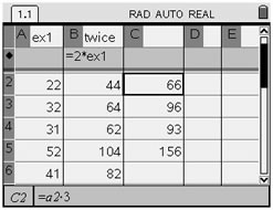
Filling Columns: Suppose we want the first cell in column C to be 30, but we want the next 4 cells to be 3 times their corresponding values in column A.
1. Enter the first cell value of 30 directly.
2. Now, in cell C2, type the formula =A2*3.
3. Press MENU, #3 Data, #3 Fill Down.
4. Now, arrow down to cover the number of cells you wish to fill. You will see a dotted line around the cells. Hit ENTER.
5. The cells that were highlighted will repeat the pattern set by the formula.
|
|
Selecting a Column (or Row): To select a column, press  and arrow down to highlight all of the cells you wish to capture. Now, the cells can be cleared, copied, moved, etc. and arrow down to highlight all of the cells you wish to capture. Now, the cells can be cleared, copied, moved, etc.
Copy:  +C +C |
Paste:  +V +V |
|
|
Working with a Block of Cells: Find the "mean" of cells A4, A5, B4, and B5 and place the answer in D1.
1. Highlight cell D1.
2. Type the formula = mean(A4:B5)*1.
You can find "mean" in the Catalog,  . For the block of cells, start with the upper left cell, and finish with the lower right cell. Multiplying by 1. (don't forget the decimal) will force the answer to be a decimal approximation. . For the block of cells, start with the upper left cell, and finish with the lower right cell. Multiplying by 1. (don't forget the decimal) will force the answer to be a decimal approximation.
3. The answer appears in cell D1. |
|
One Variable Statistics:
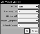
Press  , #4 Statistics, #1 Stat Calculations, and choose #1 One-Variable Statistics. , #4 Statistics, #1 Stat Calculations, and choose #1 One-Variable Statistics.
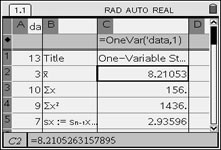
The choice "Open Variable Statistics" yields the following results back to the spreadsheet columns. One column will "label" these values, while the following column contains the actual values.
|
= mean |
|
= the sum of the data |
|
= the sum of the squares of the data |
sx |
= the sample standard deviation |
|
= the population standard deviation |
n |
= the sample size (# of pieces of data) |
MinX |
= the smallest data entry |
|
= data at the first quartile |
MedianX |
= data at the median (second quartile) |
|
= data at the third quartile |
MaxX |
= the largest data entry |
SSx |
= the sum of squared deviations of x from the
mean of x. |
|

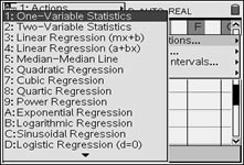
When prompted for the
number of lists, enter 1.
|
|


![]()